How a Differential Pressure Transmitter Works (2026 Guide)

A plant engineer once called us after his steam flow reading jumped 8% overnight. No leaks, no valve position changes, no maintenance logs flagged. His differential pressure transmitter had drifted at zero under high static pressure — a behavior the datasheet mentions in one line, and most English-language guides skip entirely. That kind of failure is why understanding how a DP transmitter actually works matters more than memorizing a spec sheet.

A differential pressure transmitter measures the pressure difference between two points (the high-side and low-side process taps), converts that ΔP into an electrical signal via a capacitive, diffused-silicon, or resonant-silicon sensor, and outputs a 4-20 mA signal proportional to the measured range.

Below we walk through the full loop: the physics of ΔP sensing, the three competing sensor technologies and when to pick each, how static pressure and temperature affect accuracy in the field, how ΔP converts to 4-20 mA, and the 3-valve manifold commissioning sequence that most teams get wrong on the first cold startup.

What Is Differential Pressure (ΔP) and Why Measure It?

Differential pressure is just one number — P_high minus P_low — but that single number tells you things a plain absolute-pressure gauge never could. Four process tasks rely on it almost exclusively:

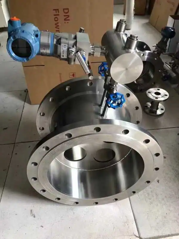
Flow across a primary element. When fluid passes through an orifice plate, Venturi tube, or flow nozzle, the pressure drop across it follows ΔP = K·Q² (where Q is volumetric flow rate). A DP transmitter is the only practical way to read that drop continuously.

Liquid level in a closed tank. The hydrostatic head of the fluid creates a static ΔP between a bottom tap and a top reference tap. A DP transmitter translates that head directly into level — independent of tank shape once you calibrate.

Filter or strainer health. A clean filter has a predictable ΔP; as it clogs, ΔP rises. You get a maintenance signal without opening the housing.

Pump performance. ΔP across the pump (discharge minus suction) tells you whether the pump is making its rated head.

Process task	What ΔP gives you	Typical range
Orifice flow	Square-root of volumetric flow	0–25 kPa to 0–100 kPa
Tank level	Linear liquid height	0–10 kPa to 0–100 kPa
Filter health	Clogging signal	0–50 kPa
Pump ΔP	Pump head verification	0–1 MPa to 0–4 MPa

For the full product lineup across these applications, see our differential pressure transmitter category.

The Working Principle, Step by Step

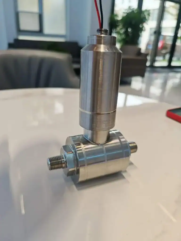
Every DP transmitter has one job: take a mechanical pressure difference and turn it into a proportional electrical signal. The way that happens is worth walking through, because each piece matters when something drifts in the field.

Inside a differential pressure transmitter, the high-side and low-side process pressures first arrive at two isolating diaphragms — 316L stainless for most duties, Hastelloy for chlorides, tantalum for very aggressive service. These outer diaphragms keep the process fluid out of the sensing element. Behind each one sits a thin layer of fill fluid, usually silicone oil (DC200) for general service, or fluorinated oil — Krytox or Halocarbon — for oxygen and chlorine applications where a hydrocarbon oil leak would be catastrophic.

That fill fluid carries the pressure inward to a central sensing diaphragm, which deflects by an amount proportional to the ΔP between the two sides. Depending on design, the sensing element — capacitive, diffused silicon, or resonant silicon — converts that deflection into a change in capacitance, resistance, or resonant frequency. A microprocessor then reads the raw signal, linearizes it, compensates for temperature, and scales it to 4-20 mA. On top of that current signal, most modern units also overlay a HART digital signal on the same two wires.

One less-obvious benefit of “differential” sensing: common-mode errors — the background static pressure, for instance — largely cancel at the diaphragm itself, not in software. You get noticeably better accuracy from a real DP transmitter than from subtracting two absolute gauge readings on a computer, because the cancellation is physical.

Typical performance across the category: spans from 0–1 kPa up to 0–40 MPa, accuracies from ±0.075% to ±0.25% of calibrated span, and service temperatures from −40°C to +85°C for the electronics (process fluid can go hotter with remote seals).

For the signal conversion side of the loop, our 4-20 mA current loop guide covers wiring, power budget, and HART troubleshooting.

Three Sensing Technologies Compared

Here is where most English DP guides stop short — they describe “a diaphragm and some electronics” without naming which technology is inside. In practice there are three, and picking the wrong one will cost you either money or accuracy.

Capacitive Sensing

Two rigid capacitor plates sit on either side of a flexible metal diaphragm. When ΔP deflects the diaphragm, capacitance rises on one side and drops on the other; the ratio between the two is your ΔP reading. Rosemount 3051 and most legacy refinery differential pressure transmitters use this architecture, and forty years of field service have made it the default choice for high-stakes duties.

Capacitive units shine when static pressure gets extreme or when the process is hot enough to require remote diaphragm seals. The trade-off is slightly higher temperature drift than silicon and a higher assembly labor cost — which is why you rarely see a capacitive unit under $400. Pick it for high-pressure pipelines, refinery compressor suction/discharge, or any service above 10 MPa line pressure.

Diffused Silicon (Piezoresistive)

A MEMS silicon chip carries four piezoresistors diffused into its surface, wired as a Wheatstone bridge. Fill fluid presses the chip; the bridge output swings proportionally to ΔP. This is what sits inside our HM51 DP transmitter and most cost-competitive units on the market worldwide.

Cost and speed are the big wins here — 0.075% accuracy comes at a fraction of the capacitive price, and response time drops to 20–50 ms, which matters on fast flow loops. The catch is static-pressure behavior: under sustained high line pressure, the silicon chip develops a small nonlinear offset that has to be corrected with polynomial compensation coefficients burned in at the factory. An on-chip Pt100 handles temperature correction in the same way. When those compensations are properly characterized, diffused silicon becomes the workhorse of mid-range DP applications.

Resonant Silicon (MEMS Frequency Shift)

Two H-shaped silicon resonators vibrate near 90 kHz. ΔP stresses them asymmetrically — one resonant frequency rises, the other falls, and the difference is your signal. That signal is inherently digital, so there is no analog-to-digital conversion error to drift with time. Yokogawa EJA and DPharp differential pressure transmitters use this approach.

You pay for it. Resonant silicon sits at the top of the price band ($1,500 and up) and the manufacturing batch cadence is slower. What you get in return is the lowest long-term drift of any technology — 0.1% over ten years is typical — which pays back quickly on custody-transfer applications or anywhere a recalibration visit is expensive.

Side-by-Side Comparison

Metric	Capacitive	Diffused Si	Resonant Si
Accuracy (% of span)	±0.075–0.1%	±0.075–0.25%	±0.04–0.075%
Static-pressure effect (per GB/T 28474.1-2012)	≤ 0.1% / 10 MPa	≤ 0.2% / 10 MPa	≤ 0.08% / 10 MPa
Temperature effect	±0.05% / 10°C	±0.04% / 10°C	±0.03% / 10°C
Response time	100–200 ms	20–50 ms	50–100 ms
Typical price (USD)	$400–$1,200	$180–$500	$1,500–$3,500
Preferred use case	High static / big flow	Cost-sensitive / fast loops	Long-term stability / custody

One practical shortcut from Sinopec’s Beijing Design Institute, where our chief temperature engineer Ye Dong spent two decades running instrumentation design: for services above 20 MPa line pressure, capacitive wins on predictability; for fast flow loops with rapid transients, diffused silicon is the default choice; for anything on a custody-transfer ticket, resonant silicon pays its premium back within about three years through avoided recalibration visits. Those rules have held up across refinery, petrochemical, and pipeline projects for a long time.

Browse HM Series DP transmitters to see which technology fits our standard, high-temperature, and sanitary variants.

Static Pressure Effect and Temperature Compensation

This is the section that catches most engineers off guard. Every DP transmitter has a calibrated span (say, 0–100 kPa), but the entire unit may be sitting under 10 MPa of process line pressure. That background pressure is the “static pressure,” and it does affect the reading.

Static pressure effect is the zero-point shift in the transmitter’s output when line pressure changes, even if ΔP stays constant. On a 100 kPa span transmitter seeing 10 MPa static, a capacitive unit may drift 0.1% FS (= 0.1 kPa zero offset). A diffused silicon unit may drift twice that. In flow metering — where you’re already reading a small ΔP on top of a high line pressure — this is the dominant source of “phantom drift.”

The Chinese national standard GB/T 28474.1-2012 (Smart transmitters for industrial process measurement and control — Part 1) defines the static-pressure influence test and the maximum allowable drift rates shown in the table above. If you are procuring for the Chinese market or exporting to it, naming that standard in your purchase specification is a short, free way to cut downstream compliance arguments.

Temperature effect is the zero-point and span shift as ambient temperature moves. Every modern transmitter has an on-board Pt100 (or equivalent diode) that measures the sensor-module temperature and applies a polynomial correction — factory-characterized over −40°C to +85°C. On our HM51 units we see ±0.05% FS per 10°C after compensation, matching the table above.

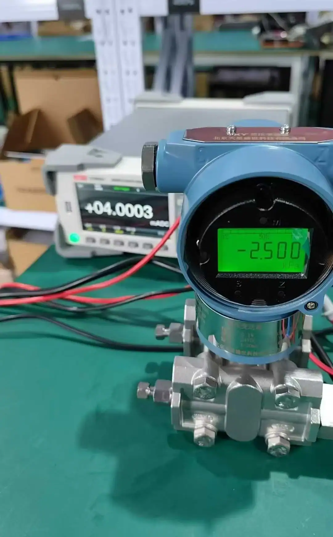
Field tip: when you commission a new DP transmitter on a high-pressure line, zero it after the line is up to operating static pressure, not before. Zeroing at atmospheric and then pressurizing the line is the single most common cause of an 8% phantom flow offset — the same failure mode from the opening of this article.

Converting ΔP to a 4-20 mA Signal

Once the sensing element produces a raw electrical signal (capacitance change, bridge millivolts, or frequency difference), the electronics board does four things:

1. Analog-to-digital conversion at 16 to 24 bits.
2. Linearization using factory-stored calibration coefficients.
3. Temperature compensation using the on-board Pt100 reading.
4. Scaling to 4-20 mA based on the configured lower range value (LRV) and upper range value (URV).

Scaling math is simple. For a 0–100 kPa calibrated span reading 60 kPa:

Output = 4 + (60 / 100) × 16 = 4 + 9.6 = 13.6 mA

Most modern DP transmitters also overlay a HART digital signal on the same two wires — a 1200 bps frequency-shift-keyed channel riding on top of the 4-20 mA current. It gives you diagnostic data, multivariable readings, and remote ranging without a separate cable.

Wiring is two-wire loop-powered (24 VDC nominal) for the vast majority of field installations; four-wire is reserved for units with integral indicators or mA-plus-frequency output for flow computers.

3-Valve vs 5-Valve Manifold Commissioning

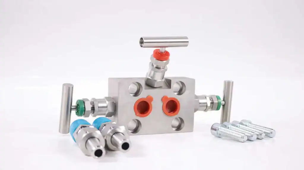
Every DP transmitter on a high-pressure line is mounted on a manifold — a valve block between the process taps and the transmitter body. A manifold lets you isolate, equalize, vent, and zero the differential pressure transmitter without shutting the line. Two variants dominate:

• 3-valve manifold: high-side isolation valve, low-side isolation valve, equalizing valve.
• 5-valve manifold: same three, plus two vent (drain/bleed) valves for flushing and zero verification.

Chemical, oil & gas, and power plants in China default to 5-valve; water treatment and HVAC default to 3-valve.

Here is the 6-step startup sequence that most English-language installation guides leave out. It comes straight out of Sinopec EPC commissioning manuals, and it is the right way to bring a DP transmitter online without zero-shock:

1. Close both isolation valves (high-side and low-side). The transmitter is isolated from the process.
2. Open the equalizing valve. Both sides of the sensor now see the same static pressure. Zero output reading should equal 4 mA (or your configured LRV).
3. Slowly open the high-side isolation valve. Watch the transmitter — you’re bringing it up to line static pressure on both sides simultaneously.
4. Close the equalizing valve. The high and low sides are now isolated from each other.
5. Slowly open the low-side isolation valve. At this point the transmitter is seeing the real process ΔP.
6. Verify zero-return. Re-open the equalizing valve briefly; output should drop to 4 mA cleanly. If it doesn’t, the sensor may have zero-shifted under static pressure — recalibrate at operating static, not atmospheric.

A common field mistake is opening the low-side isolation valve first — that slams the center diaphragm with full line pressure from only one side and can permanently shift zero. The equalize-first rule exists for a reason.

For a deeper dive with installation diagrams, see our DP transmitter manifold valve guide (coming soon).

Frequently Asked Questions

Ready to Specify a DP Transmitter?

Every application we’ve covered — flow, level, filter, pump — has a best-fit sensing technology and a best-fit span. If you have a specific application brief (process fluid, static pressure, desired accuracy, budget), we’ll recommend the right HM series model.