Pressure Sensor Temperature Compensation: How It Works
An uncompensated pressure transmitter sitting outdoors will read a different value at 5 °C than at 45 °C, even when the actual line pressure has not moved. This guide walks through what is physically happening inside the sensor, how the two distinct error modes (zero shift and span shift) are decomposed, what the ±%FS/°C number on a datasheet actually means, and the passive and active circuits engineers use to cancel the drift. We close with verified compensation specs across five HMK transmitter families, plus a short decision list for picking a unit that fits your real ambient swing.. The same compensation budget sets the floor for any precision-grade transmitter; see precision pressure sensor for the 0.1 % FS line and how thermal coefficients fit the ladder.
Why Temperature Shifts a Pressure Reading
A pressure sensor is a transducer made of physical things: a diaphragm, four bridge resistors on a silicon or ceramic substrate, an oil fill, an electronics board. Every one of those parts is temperature-sensitive in some way. The diaphragm’s Young’s modulus drops as it warms. The piezoresistive coefficient of the silicon strain gauges changes by about 0.2 %/°C. The fluid trapped behind the diaphragm expands. Even the solder joints and traces on the analog board contribute their own ppm-level drift.
Net effect: the same 100 kPa applied to the diaphragm produces a different output voltage at 5 °C than at 45 °C. With a typical uncompensated piezoresistive sensor, the gap is roughly 1–2 % of full scale across that 40 °C swing — large enough to push a Class 0.25 transmitter out of spec by mid-morning. The mechanical analog of this problem is even cleaner to picture: a Bourdon-tube gauge has twelve cooperating parts, every one of them metallic, every one expanding with heat. Compensation is what turns those uncoordinated drifts back into a reading you can trust.
Two Errors in One: Zero Shift vs Span Shift
Datasheets always specify temperature drift as two numbers, not one, because the error is structurally two different things stacked on top of each other.
Zero shift, sometimes labelled TZS or “thermal zero error”: at zero applied pressure, the output drifts away from its 0 V or 4 mA calibration point as temperature changes. It is essentially additive — every reading is offset by the same amount across the full pressure range at that temperature. Zero shift is most often roughly linear in T, and the spec is written as ±%FS/°C.
Span shift, sometimes labelled TSS or “thermal sensitivity drift”: at full pressure, the gain of the bridge changes. The whole transfer function tilts: at 5 °C the sensor might output 4–20 mA across 0–100 kPa; at 45 °C it might output 4.2–19.7 mA across the same range. Span shift is multiplicative, and on cheaper sensors it is non-linear in T.
We see the two errors decouple because they have different physical causes. Zero shift is dominated by mismatch in the four bridge-resistor TCRs. Span shift is dominated by the temperature dependence of the silicon piezoresistive coefficient. A sensor can be excellent at one and poor at the other; an honest datasheet specifies them separately.
Inside the Wheatstone Bridge
To see why TZS and TSS behave differently, look at the circuit doing the work.
A piezoresistive pressure sensor is a four-resistor Wheatstone bridge etched into a silicon diaphragm. When pressure deflects the diaphragm, two of the resistors stretch (R rises) and two compress (R falls), which unbalances the bridge and produces a voltage at the output node proportional to applied pressure.
When the sensor warms uniformly, all four resistors gain resistance at the same temperature coefficient (TCR), and to first order they cancel at the bridge-output node. So if every R drifted at exactly the same rate, you would have no zero shift. In practice, manufacturing tolerances leave a residual TCR mismatch of a few hundred ppm/°C between resistors, and that mismatch is what drives TZS.
The span behaves differently. The piezoresistive coefficient itself, the constant relating ΔR/R to applied stress, falls roughly 0.2 %/°C in p-doped silicon. So the bridge gets less sensitive as it warms, even when every resistor is perfectly matched. That gain droop is what the active or passive comp circuit has to flatten out.
Reading the Datasheet: Decoding ±%FS/°C
The compensation spec on a datasheet packs a lot of decisions into a few notations. Below is what each one means in practice.
| Notation on datasheet | What it means | Worked example on a 100 kPa sensor |
|---|---|---|
| ±0.01 %FS/°C TZS (typ) | Zero output drifts 0.01 % of full scale per °C, typical | 30 °C swing → ±0.3 % FS = ±0.3 kPa zero shift |
| ±0.02 %FS/°C TSS (max) | Span gain drifts up to 0.02 %FS/°C in the worst-case unit | 30 °C swing at full scale → up to ±0.6 % FS = ±0.6 kPa |
| ±1 % FS over 0…50 °C | Total error band including TZS + TSS + non-linearity over a stated range | At any point in 0–50 °C, total error stays inside ±1 % FS |
| Compensated range | Temperature window inside which the comp circuit is active and the spec is valid | e.g., -10 …+ 60 °C |
| Operating range | Wider window the sensor will survive without permanent damage | e.g., -40 …+ 85 °C |
Two numbers worth holding in your head. First, the compensated range and operating range are not the same thing. A sensor will keep producing readings outside its compensated band, but the reading is no longer guaranteed to its accuracy spec. Second, “typical” and “max” can differ by 10x on the same line; if you are writing a contract spec, write the max.
IEC 60770-1:2010 defines the test procedure for both numbers — three temperatures inside the compensated range, ten cycles per temperature, hold time long enough for the whole assembly to thermally stabilise. The Chinese equivalent, GB/T 28474-2012, follows the same structure with slightly tighter rest times.
Passive Compensation: All-Analog, No Power
The oldest and still most common compensation scheme is all in the analog domain. Several techniques are usually combined.
The first is bridge-resistor matching. During wafer-level manufacturing, the four bridge resistors are laser-trimmed so that their TCRs converge to within a few tens of ppm/°C. This alone eliminates most of the zero shift you would otherwise see.
The second is a temperature-sensitive resistor placed in series with the bridge excitation. As the bridge warms and its sensitivity drops, the series resistor warms in step and reduces excitation voltage just enough that the falling sensitivity is offset by rising drive. This kills span shift to first order. The series resistor is typically a thin-film NTC (negative temperature coefficient) element on the same substrate.
The third is a voltage-divider network for residual zero offset. A second pair of carefully selected fixed resistors is added between the bridge and the output stage, sized so that the small residual TCR mismatch is bucked out by an opposite-direction divider drift.
Passive compensation has three things going for it: it is cheap, it is reliable (no firmware), and it draws no extra power. It has one big limitation. It only flattens linear-in-T errors, and only inside the compensated band. Push the sensor outside that band, or expose it to a non-linear thermal effect, and the passive network has nothing left to give. Most general-purpose transmitters in the field — including HMK’s HM50 Anti-Corrosive Pressure Transmitter at ±0.015 %FS/°C — rely on this approach.
Active Compensation: A Built-in Temperature Sensor and a Polynomial
The newer alternative is to measure temperature directly, digitise both signals, and let firmware do the math. A modern smart transmitter contains a primary pressure sensor, a secondary temperature sensor (often a diode or RTD on the same die), an analog front-end with two ADC channels, a microcontroller, and a non-volatile memory holding a calibration matrix.
At calibration time, the unit is exposed to a grid of pressure and temperature points — typically 5 × 5 or 7 × 7. The microcontroller logs the raw bridge output at each grid point and stores a two-dimensional polynomial fit. In service, the device reads pressure and temperature simultaneously, looks up the polynomial coefficients, and applies the correction before it puts a value out on the 4–20 mA loop or HART telegram.
Active compensation buys three things passive cannot. It can correct non-linear-in-T errors, because the polynomial has cross-terms. It can compensate over the full operating range, not just the calibrated one, because the firmware extrapolates. And it can bring the spec down to ±0.0075 %FS/°C territory, an order of magnitude better than analog tricks.
The HMK HM3051 Smart Differential Pressure Transmitter implements this approach with a 2D calibration matrix and HART communication. Its specified zero and span temperature influence each work out to about ±0.0018 %FS/°C, calculated from the published ±0.1 %/55 °C figure — three to five times tighter than its passive-comp peers.
Standards That Govern Compensation Testing
Four written standards specify how a compensation claim has to be proven. A vendor that does not cite at least one of them is making it up.
| Standard | Region | What it covers | Key clause for TC |
|---|---|---|---|
| IEC 60770-1:2010 | Global | Performance evaluation methods for industrial-process transmitters | §6.3 thermal effects on zero and span |
| IEC 60770-2:2017 | Global | Inspection and routine-test methods, including thermal cycling | §5.4 thermal performance verification |
| GB/T 28474-2012 | China / SE Asia | General specification for pressure transmitters | §4.5 temperature influence test |
| JJG 882-2019 | China metrology | Periodic verification of pressure transmitters in service | §6 retest interval and pass/fail at temperature |
These four standards line up: a transmitter tested to IEC 60770-1 also satisfies the equivalent GB/T 28474 procedure with no rework. JJG 882-2019 is the only one that prescribes how often you have to re-verify the unit after install, and the answer is one year for general process service or six months for safety-critical applications.
For traceability beyond the test, NIST’s pressure metrology group anchors the dead-weight tester chain that calibration labs reference globally, and the lab itself has to be accredited under ISO/IEC 17025 for the certificate to be admissible in a procurement contract.
What Failure Looks Like in the Field
Two anonymised cases we worked on with HMK customers show what under-compensation actually costs.
The first is a Southeast Asian refinery feedstock-line transmitter, mounted outdoors with no sun shield. The original unit was an uncompensated piezoresistive transmitter rated ±0.5 % FS at room temperature. Field measurements showed a 1.5 % FS reading swing between dawn (5 °C) and noon (45 °C). The control loop had its alarm bands wide enough to absorb the swing, but the operators had effectively given up trusting the gauge for trim decisions. Replacing the unit with an actively-compensated transmitter dropped the diurnal swing to 0.15 % FS, and operations got their trim margin back.
The second case is a Mumbai fertiliser plant ammonia line. The transmitter was a quality unit specified ±0.02 %FS/°C across a -10 to +50 °C compensated range. Plant ambient routinely exceeded +60 °C in the hot season. The unit kept reading, but it was running outside its compensated band, and the apparent 2 % FS drift the team blamed on instrument failure was actually the device behaving exactly as its spec described — outside spec range. The fix was to move the transmitter to a conditioned cabinet, then later swap to a unit with a compensated range that matched real ambient + 10 °C of margin. Lesson: pick the compensated band of the device to envelope the actual temperature swing the unit will see, not the published “operating” range.
A related but distinct failure mode shows up in liquid-level loops: when the process fluid’s density drifts with temperature (a different problem from the sensor temp drift this article covers), even a perfectly compensated transmitter reads the wrong level. The hub article on hydrostatic level measurement covers that case, including specific-gravity correction strategies.
HMK Compensated Transmitters at a Glance
Five HMK families cover the typical compensation envelopes you find on a process plant. The numbers below come straight from each unit’s datasheet on hammok-tech.com.
| HMK family | Sensing element | TZS (typ) | TSS (typ) | Compensated range | Operating range | Best for |
|---|---|---|---|---|---|---|
| HM22 High-Accuracy | Piezoresistive Si, hybrid passive + digital trim | ±0.01 %FS/°C | ±0.01 %FS/°C | -20 to +60 °C | -40 to +85 °C ambient | Aerospace, lab, calibration applications where TC dominates the spec budget |
| HM3051 Smart DP | Capacitive Si, oil-filled | ±0.0018 %FS/°C (≈ ±0.1 %/55 °C) | ±0.0018 %FS/°C | -29 to +93 °C electronics | -40 to +315 °C with high-T fill | Smart DP service: HART, SCADA, 5×5 cal matrix |
| HM50 Anti-Corrosive | Piezoresistive Si, all-stainless wetted | ±0.015 %FS/°C (combined zero + span) | combined with zero | -10 to +60 °C | -40 to +85 °C | Sour service, chloride brines, oil-fill-incompatible media |
| HM80 High-Temp Melt | Sapphire diaphragm + capillary | ±0.03 %FS/°C typ (±0.05 max) | combined | per spec envelope | -20 to +80 °C electronics, +350 °C max media | Plastic extrusion, polymer melt, injection moulding |
| HM28 Sapphire | Sapphire piezoresistive | overall accuracy ≤ ±0.1 % FS across compensated range | (combined; not separately published) | -40 to +120 °C, extended +200 °C variant | -65 to +200 °C | Aerospace, nuclear, deep-sea, radiation-hard service |
What the numbers tell you. If your line is room-temperature and the budget is tight, an HM50 at ±0.015 %FS/°C is plenty. If you are writing a control loop where TC dominates, the HM22 at ±0.01 %FS/°C is the value pick. If you need both smart digital comm and a wide thermal envelope, the HM3051 wins on both axes. The HM80 and HM28 take over when the process media itself is hot enough that the sensor needs sapphire.
FAQ
What does ±0.01 %FS/°C mean on a pressure sensor datasheet?
It means the sensor’s reading drifts up to 0.01 % of full scale for every degree Celsius temperature change inside its compensated range. On a 100 kPa unit, a 30 °C ambient swing produces up to 0.3 % FS or 0.3 kPa of drift. The figure is usually given separately for zero shift and span shift; if the datasheet gives only one combined number, assume the worst case is twice that.
What is the difference between compensated range and operating range?
The compensated range is the temperature window inside which the sensor’s accuracy spec is valid. The operating range is the wider window the sensor will survive without damage but without an accuracy guarantee. A unit rated -10 to +60 °C compensated and -40 to +85 °C operating will produce readings at -20 °C, but the readings carry no spec backing — pick the compensated range to envelope your real ambient.
Active vs passive temperature compensation: which one should I pick?
Pick passive (analog) when ambient stays within a 60–80 °C band, when accuracy at ±0.5 % FS or wider is acceptable, and when no smart-comm is needed. Pick active (digital) when accuracy below 0.25 % FS is required, when ambient swings outside a single band, when you want HART or SCADA, or when the application has non-linear thermal effects passive cannot handle. Hybrid units (HMK HM22, HM50) use passive for the bulk drift and a small digital trim for the residual.
Why does my pressure reading change in the morning vs afternoon?
Almost always uncompensated or under-compensated TC. A uncompensated outdoor transmitter will show 1–2 % FS swing across a typical 25 °C diurnal cycle. Verify by logging the transmitter output and ambient temperature for 24 hours and looking for correlation. If ambient is the cause, either fit a sun shield and conditioned enclosure, or replace with a unit whose compensated range envelopes your real temperature swing.
Do I need a compensated sensor for indoor process applications?
Indoor process plants are not as benign as they look. A boiler room can swing 10 °C between night and shift change; a server room or HVAC plant has duty cycles that introduce 5 °C steps; a pharma cleanroom has stable ambient but the process media itself is sometimes 60 °C above ambient. Any of these will show up as drift on an uncompensated unit. The general rule: if you are spec’ing a transmitter at Class 0.25 % FS or tighter, you need temperature compensation, indoor or out.
If your application sees ambient swings or process-media temperature outside 0–50 °C, the HM3051 Smart DP holds ±0.0018 %FS/°C through its full compensated range, and the HM80 High-Temp Melt Pressure Transmitter extends compensation to +350 °C process media. For everything in between, the HM22 High-Accuracy and HM50 Anti-Corrosive families round out the line.
Related reading: Temperature compensation requirements vary by industry. See pressure transducer applications by industry for which transducer fits hydraulic, HVAC, oil and gas, sanitary, and lab service.
Related: Above the compensated band, temperature compensation alone is not enough; for furnace, boiler and steam service step up to a dedicated high-temperature pressure transducer or a remote seal.